Chapter 2

The Law of Demand and the Theorem of Exchange

 

I. Indifferent Curve Analysis (Ordinary Concept of Utility)

 

A. Introduction

 

1) What is a good?

 

A good is an entity at least one person prefers to have some than none.

       

2) What is a bad?

       

A bad is an entity which less is preferred to more and none is preferred to some.

 

3) What is a neuter?

 

A neuter is an entity of which an individual is indifferent between having more or less. That is , it is neither a good nor a bad.

 

B.    Assumptions for Ranking of different options    

 

1) Axiom of comparison

 

Given different bundles of commodities, Commodity A and Commodity B, a rational consumer is able to compare them.

 

For example: If there are 2 commodities, Commodity A and Commodity B, a consumer will say: AfB, BfA or A~B.

                                      

2) Axiom of transitivity

 

If AfB, BfC , then AfC.

 

 

3) Both Commodity X and Commodity Y are economic goods. For an economic good, more is preferred to less.

 

4) Postulate of substitution.

 

An individual is willing to trade some of a good for another good.

 

5) Postulate of Diminishing Marginal Rate of Substitution.

 

C.    Utility

 

1) What is utility?

 

Utility is an arbitrary assignment of index (or number) for ranking options. Utility means rank ordering of preference.

 

For example: CfAfB

 

Option	Combination of Good X & Good Y	Utility
A	5X & 6Y	2nd
B	3X & 4Y	3rd
C	7X & 7Y	1st

 

2)          What are the postulates of utility maximization?

 

An individual always wants to attain a higher indifference curve.

 

If the postulate of utility maximization can give testable implications on human choice, it is useful.

 

D.  What is an indifference map 

 

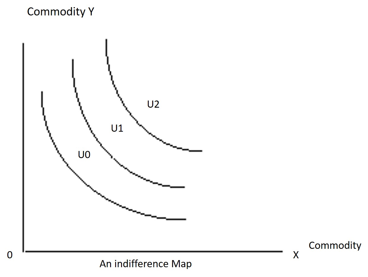
The preference of an individual is represented by a set of indifference curves. An indifference map is made up of indifference curves

 

An Indifference map shows the preference or taste of an individual on 2 commodities, Commodity X and Commodity Y.

 

 

E.     What is an indifference curve?

 

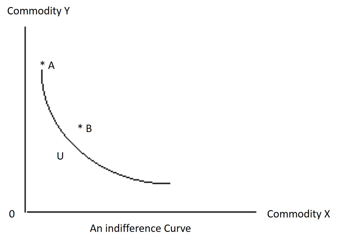
An indifference curve is a curve showing different combinations of two goods  that an individual finds them equally preferable. That is, it is a curve showing   different combinations of two goods with the same utility level.

 

Points on the same indifference curve give the same level of utility, i.e. they have the same rank ordering of preference or they are equally preferable to each other.

 

An individual will be indifferent among all possible combinations on the same indifference curve. If Point A and Point B are indifferent, that is with the same level of utility. They must be on the same indifference curve.

 

           

F.          The properties of indifference curves

 

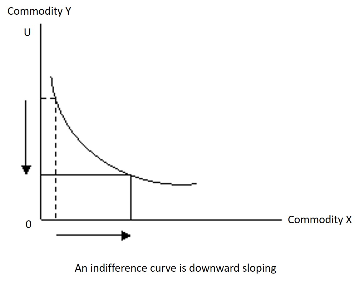
1) An indifference curve is downward sloping.

 

When the amount of Commodity Y is decreased, the amount of Commodity X must be increased due to opportunity cost and vice versa. So the indifference curve is downward sloping.

 

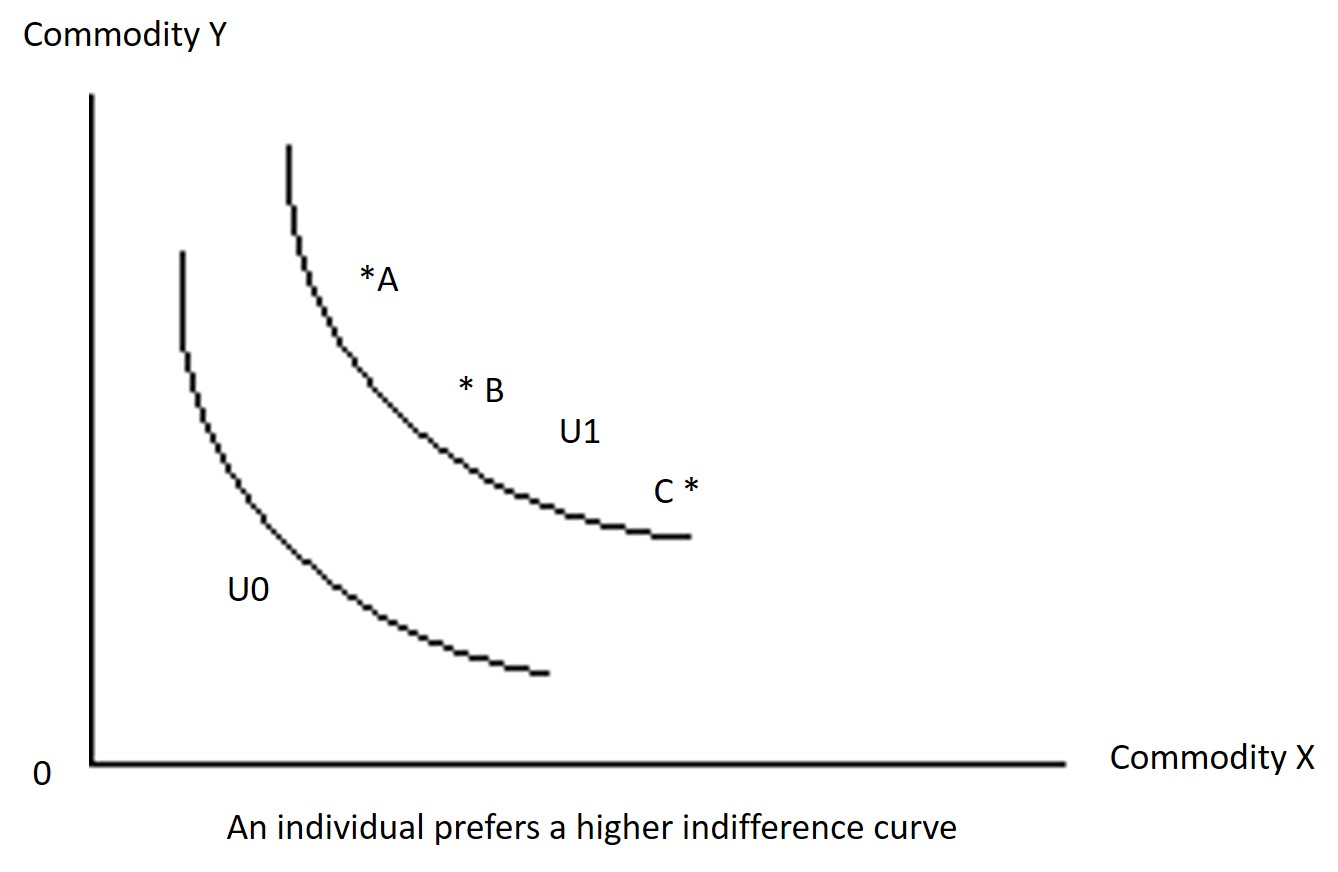
2) Indifference curves that are further away from the origin indicate a higher level of utility.

 

Individuals prefer points on a higher indifference curve. Combination B is prefer to Combination A since B has more units of Commodity X. Combination B and Combination C are indifferent since they are on the same indifference curve. According to the axiom of transitivity, it implies that C is prefer to A.

 

 

3)     Indifference curves cannot intercept.

 

       

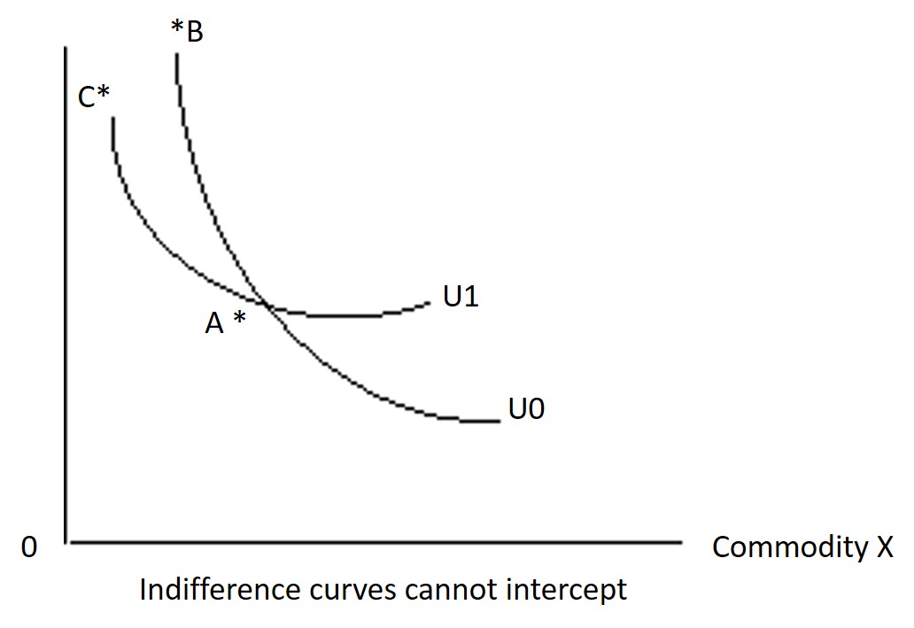
                        If indifference curves intercepted, the axiom of transitivity will be violated.

 

                        Since        A~B

A~C

                That is     B~C

                        But          BfC

        Therefore, it is inconsistent.

 

4)     Indifference curves are convex to the origin.

 

a) What is marginal rate of substitution (MRS)?

 

MRSxy is the maximum amount of Commodity Y an individual is willing to give up for an additional unit of Commodity X, holding utility unchanged.

 

MRSxy = DY/ DX = (Y₁ – Y₂)/(X₁ – X₂)

 

MRSyx = DX/ DY = (X₁ – X₂)/(Y₁ – Y₂)

 

For example: MRSxy = (4 – 2)/(2-3) = -2. That means an individual is willing to give up to 2 units of Commodity Y in order to get 1 extra unit of Commodity X while his utility remains constant. The negative sign indicates the inverse relationship between Commodity X and Commodity Y.

 

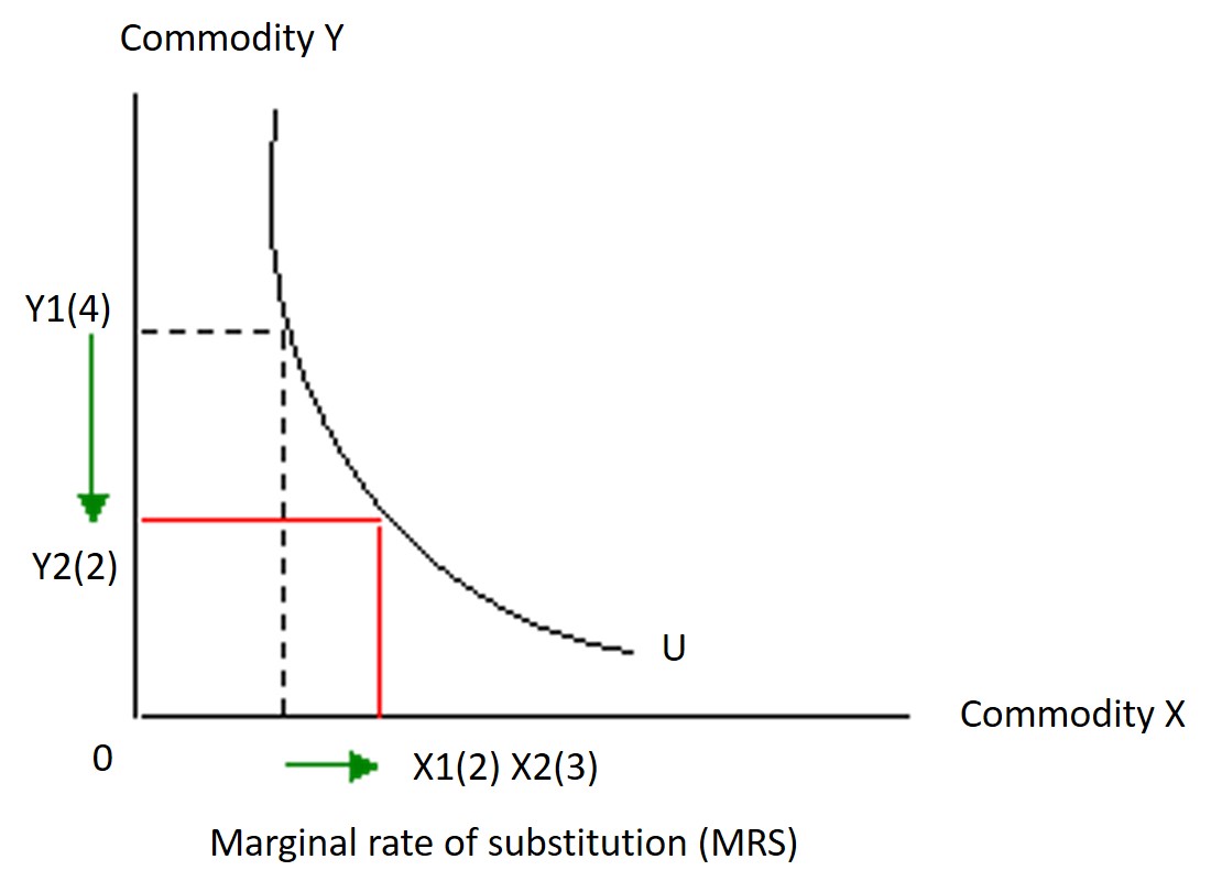
If the change in Commodity X is very small, then the change occurs at a ‘point’ on the indifference curve. Thus, the MRSxy at that point is measured by the slope of the tangent to the indifference curve. Then MRSxy = dy/dx.

 

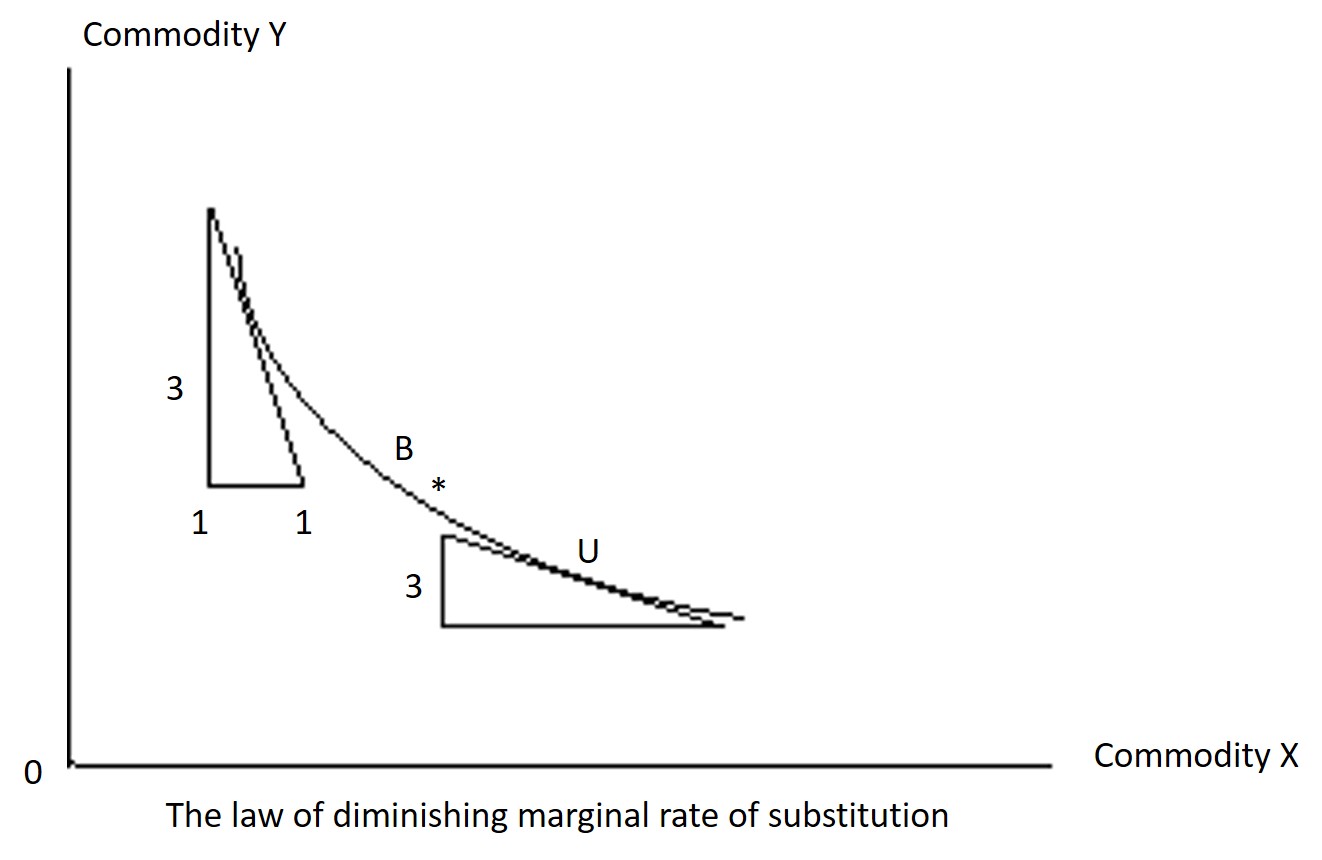
b) Why an indifference curve is convex to the origin?

 

Indifference curves are usually convex, based on the assumption of diminishing marginal rate of substitution.

 

                                What is the law of diminishing marginal rate of substitution (DMRS)?

 

DMRS asserts that the maximum amount of other goods (say Commodity Y) that an individual is willing to give up in order to obtain an additional unit of a good (say Commodity X)will always diminish.

 

The indifference curve will become flatter and flatter when more and more commodity is acquired.

 

Since an indifference curve is convex, its slope (MRSxy) becomes smaller and smaller when an individual moves down. For Example: MRSxy at Point A = 3 and MRSxy at point B = 1/3.

 

 

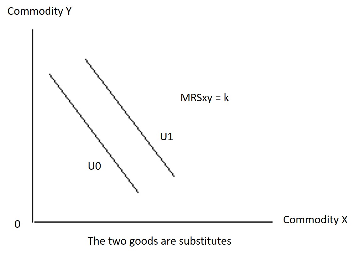
1)  The indifference curves are straight lines

 

The 2 commodities are prefect substitutes. The MRSxy is constant. If both Commodity X and Commodity Y are goods, then U₁＞U_0. If both Commodity X and Commodity Y are bads, then U₁＜U_0. The postulate of DMRS is violated

 

 

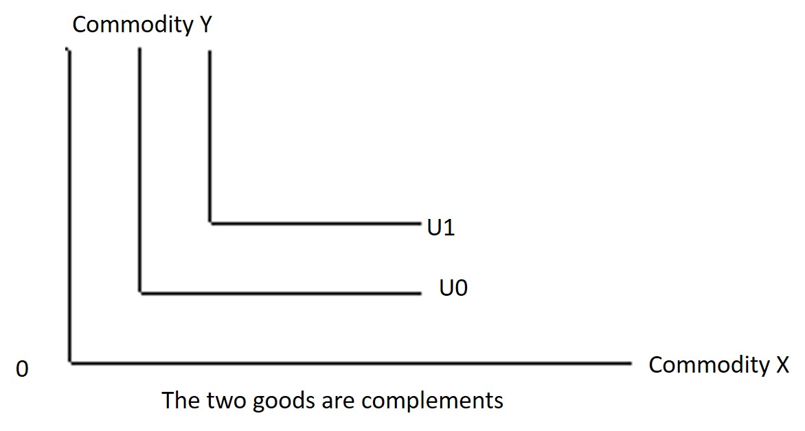
The 2 commodities are perfect complements. MRSxy is defined at the vertex. If both Commodity X and Commodity Y are goods, then U₁＞U_0. If both Commodity X and Commodity Y are bads, then U₁＜U_0.

 

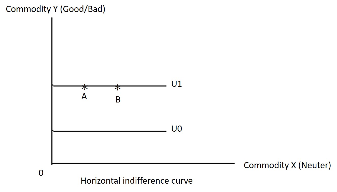
3)  The indifference curves are horizontal straight lines

 

Commodity X is a neuter. Commodity Y is a good or bad. Since Commodity X is a neuter, more is indifferent to less. So Point A and Point B lie in the same indifference curve.

 

If Commodity Y is a good, then U₁＞U₀. Given a certain quantity of Commodity Y, an individual is not willing to substitute any Commodity Y for Commodity X. If he gives up a little bit of Commodity Y, his utility level falls. That is he will be on a lower indifference curve.

 

If Commodity Y is a bad, then U₁＜U₀.

                                               

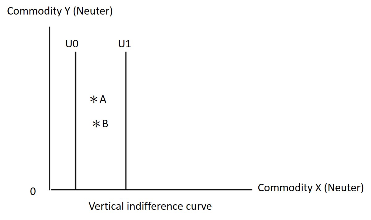
Commodity Y is a neuter. Commodity X is a good or bad. Since Commodity Y is a neuter, more is indifferent to less. So Point A and Point B lie in the same indifference curve. If Commodity X is a good, then U₁＞U₀. If Commodity X is a bad, then U₁＜U₀.

 

         

 

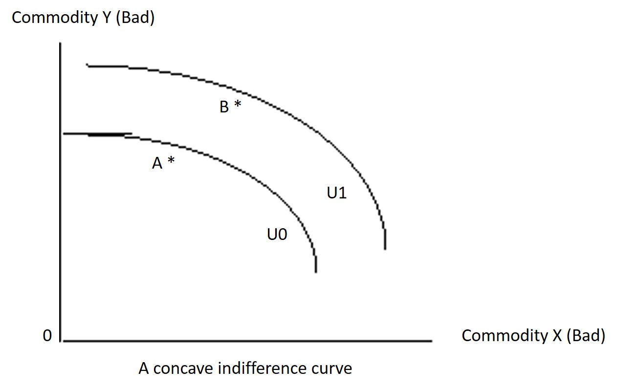
a) Both Commodity X and Commodity Y are bads.

 

Since Commodity X and Commodity Y are bads, so less of them are preferred to more. So Combination A is preferred to Combination B. Then U₀＞U₁.

 

The law of diminishing marginal rate of substitution holds

 

 

b) Both Commodity X and Commodity Y are goods.

 

Since Commodity X and Commodity Y are goods, so more of them are preferred to less. So Combination B is preferred to Combination A. Then U₁＞U₀.

 

It implies increasing marginal rate of substitution.

 

6) The indifference curves are upward sloping

 

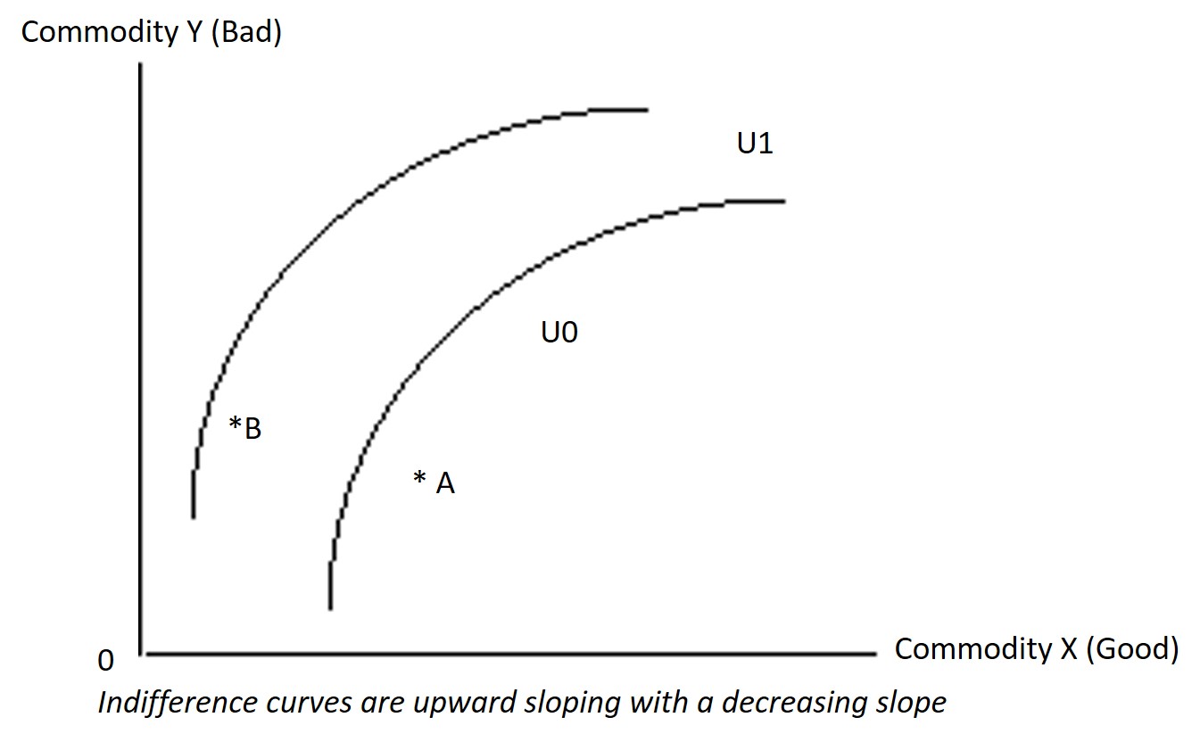
a) The indifference curves are upward sloping with a decreasing slope

 

Commodity X is a good. Commodity Y is a bad. Utility increases when the amount of a good is increased, but falls when more of a bad is obtained. Utility will be constant if the increase in a bad is accompanied with an increase in the quantity of a good.

 

Combination A and Combination B have the same amount of Commodity Y, but Combination A has more Commodity X, so it is preferred. Then U₀＞U₁.

 

 

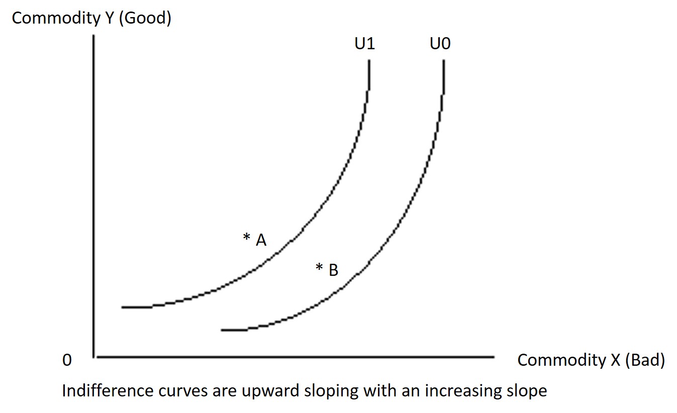
b) The indifference curves are upward sloping with an increasing slope

 

Commodity Y is a good. Commodity X is a bad. Utility increases when the amount of a good is increased, but falls when more of a bad is obtained. Utility will be constant if the increase in a bad is accompanied with an increase in the quantity of a good.

 

Combination A and Combination B have the same amount of Commodity X, but Combination A has more Commodity Y, so it is preferred. Then U₁＞U₀.

 

 

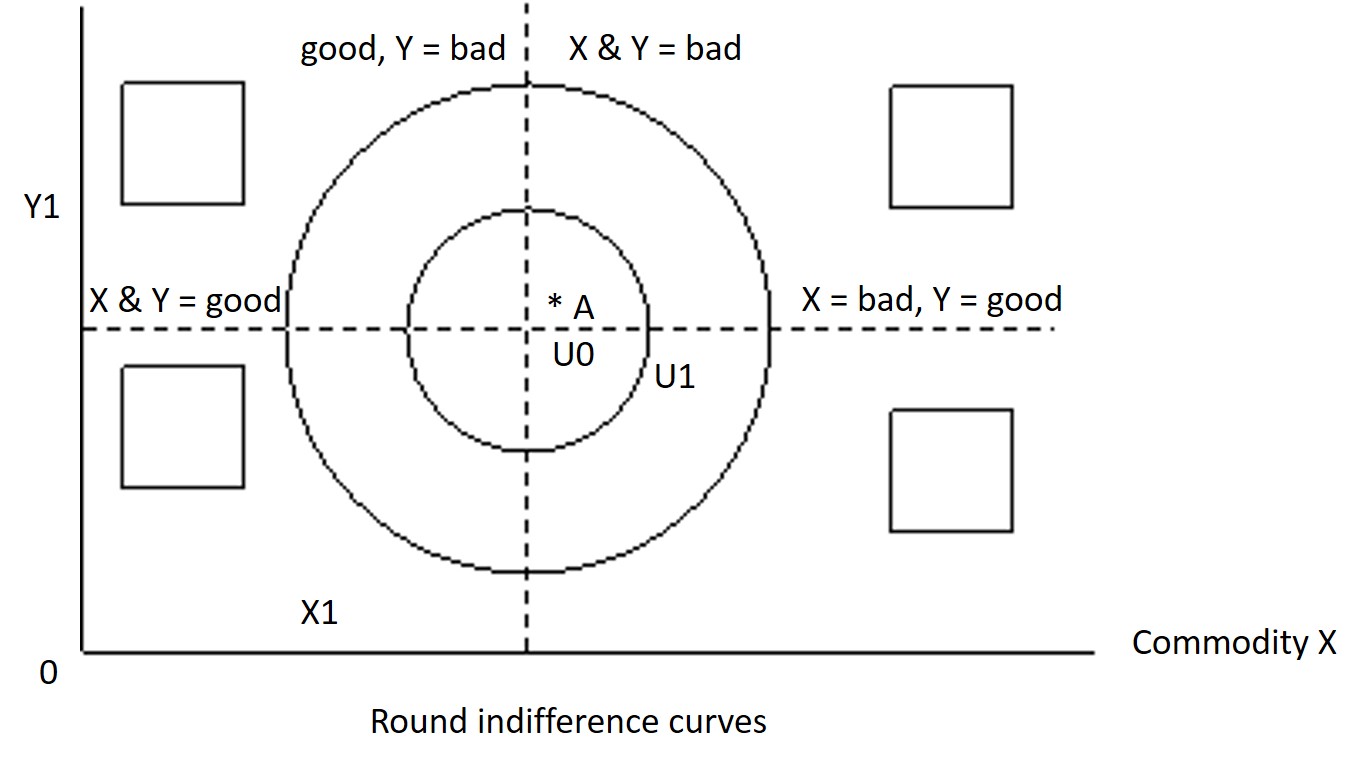
7)     The indifference curves are round

 

Commodity X and Commodity Y will change from goods to bads. Beyond X₁ and Y₁ , Commodity X and Commodity Y will change from goods to bads.

 

Combination A is the most preferred combination. Then U₀＞U₁.

 

                 

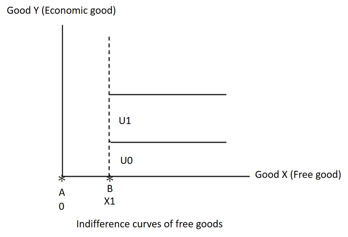
7) The indifference curves are horizontal lines starting from a certain quantity of Commodity X

 

Commodity X is a free good. Commodity Y is an economic good. Since Combination B is preferred to Combination A, Commodity X must be a good. Beyond Combination B, utility remains unchanged when the amount of Commodity X is increased.

 

Commodity X is a free good when X₁ is possessed. Then U₁＞U₀.

 

  

        H.    What is a budget line (BL)?

 

The budget line shows the maximum combinations of Commodity X and Commodity Y that an individual can afford at the prevailing prices of Commodity X and Commodity Y, given his money income.

 

The budget line defines an individual’s consumption opportunity set That is, the budget line constraints an individual’s choice.

 

I.      How to construct a budget line

 

An individual is assumed to spend all his income on Commodity X and Commodity Y.

 

                So   I = Px(X) + Py(Y)

• I = income
• Px = money price of Commodity X
• Py = money price of Commodity Y
• X = quantity of Commodity X
• Y = quantity of Commodity Y

 

Then Y₀ = I/Py and X₀= I/Px

• Y₀ = quantity of Commodity Y consumed if all income is spent on it
• X₀ = quantity of Commodity X consumed if all income is spent on it

 

                                   

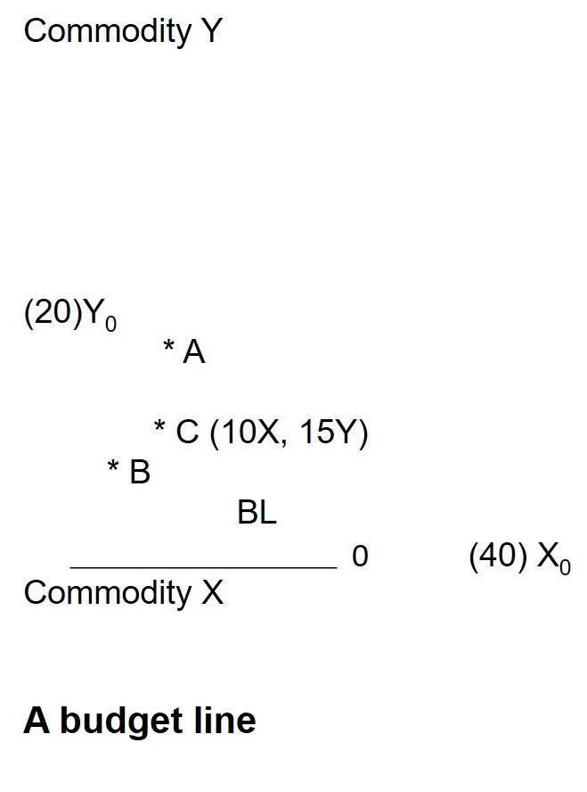
Given:

• I = Px(X) + Py(Y)
• I = $400
• Px = $10
• Py = $20
• X = 10
• Y = 15

Then: $400 = $10(10) + $20(15)

 

Since: Y₀ = I/Py. Then: Y₀ = $400/$20 = 20 units

 

Since: X₀ = I/Px. Then: Y₀ = $400/$10 = 40 units

 

Point A is not available since it is outside the budget line.

 

Point B indicates that not all income is spent since it is inside the budget line.

 

Point C indicates that all income is spent since it is on the budget line.

 

Money price and money income are the constraints of an individual’s consumption decision.

 

J.     How to find the slope of a budget line

 

The Slope of budget line   = △Y/ △X

= (Y₀ – 0)/(0 –X₀)

= –Y₀/X₀

= –(I/Py)/(I/Px)

= – Px/ Py

For example:

Since:       Slope of BL = – Px/ Py

                 Px = $10

                        Py = $20

Then

         Slope of BL = –$10/$20 = – 1/2

 

K.    How to find the relative price

               

1) What is relative price?

 

The relative price of Good X is the amount of Good Y that is required in the market to exchange for 1 unit of Good X.

 

Relative price of Good X = Px/Py

 

Relative price of Good Y = Py/Px

 

A rise in the price of one good implies a fall in the relative price of the other good.

 

For example: The initial price of Good X is $10 and the price of Good Y is $15. After an increase in the price of Good X from $10 to $20, what will happen to the relative price of Good X and Good Y respectively?

 

                                Initial relative price of Good X = Px/Py = $10/$15 = 2/3Y

 

                                Initial relative price of Good Y = Py/Px = $15/$10 = $3/2X.

 

Relative price of Good X after an increase in price = Px/Py = $20/$15

                                                                                               = 4/3Y

 

Relative price of Good Y after an increase in price = Py/Px = $15/$20

                                                                                               = 3/4Y

 

L.     What happen to the budget line, if the constraints of the budget line change?

 

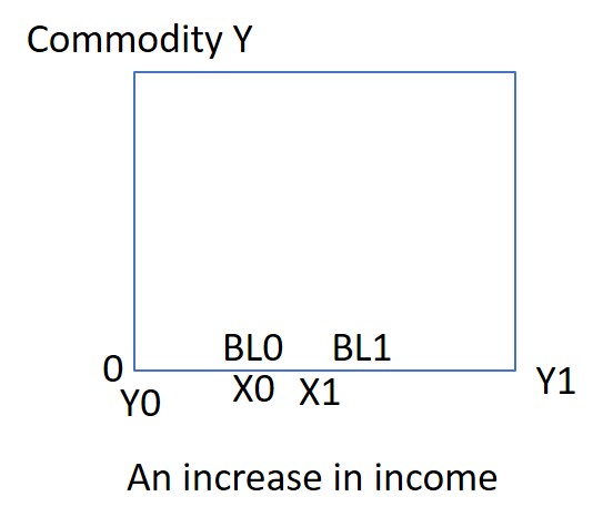
1) A change in money income

 

i) An increase in income

 

If an individual’s income increases, the budget line shifts to the right. That is, the opportunity set facing the individual increases. The individual is able to obtain more Commodity X and Commodity Y since hi/her real

 

income increases. The slope of the budget line remains unchanged.

                         

                        

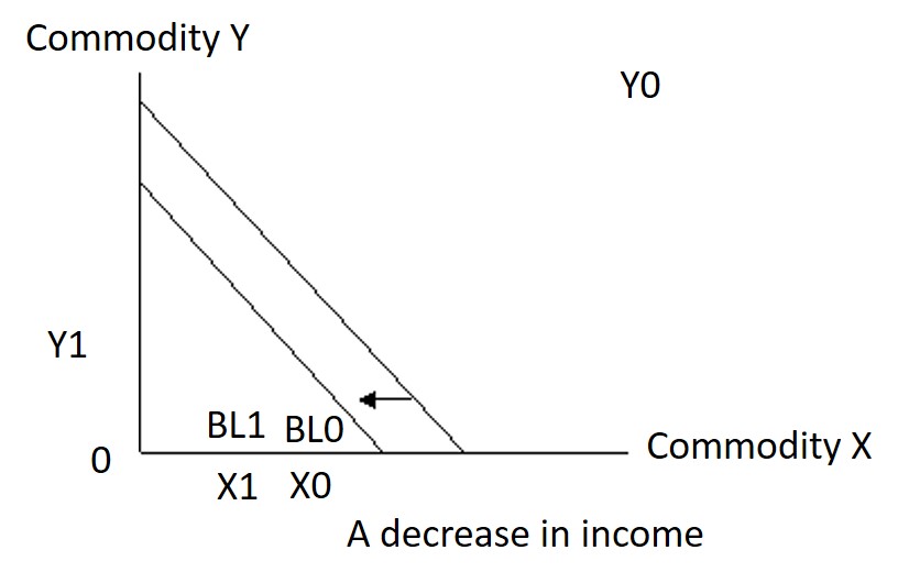
ii)     A decrease in income

 

If an individual’s income decreases, the budget line shifts to the left. That is, the opportunity set facing the individual decreases. The individual obtains less Commodity X and Commodity Y as his/her real income decreases. The slope of the budget line remains unchanged.

 

 

2) The price of a commodity changes

 

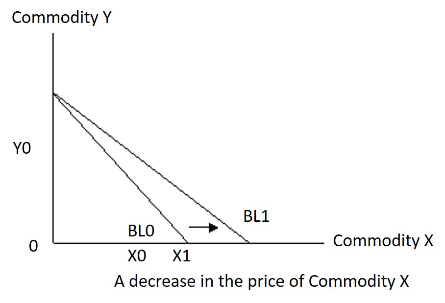
i) A decrease in the price of Commodity X

 

That is the slope of the budget line becomes smaller. The budget line rotates outward. The budget line becomes flatter. The opportunity set facing the individual increases. The individual obtains more Commodity X and Commodity Y.

 

 

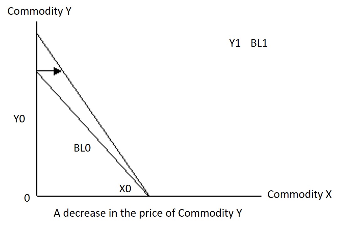
ii) A decrease in the price of Commodity Y

 

The budget line rotates outward. The budget line becomes steeper. The opportunity set facing the individual increases. The individual obtains more Commodity X and  Commodity Y.

 

 

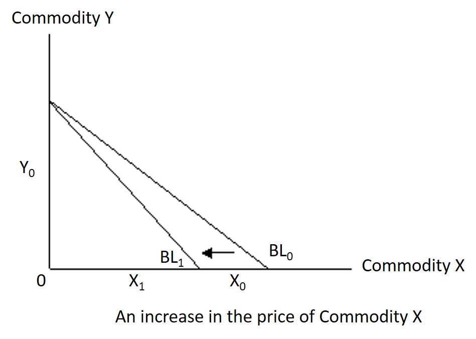
iii)           An increase in the price of Commodity X

 

The budget line rotates inward. The budget line becomes steeper. The opportunity set facing the individual decreases. The individual obtains less Commodity X and Commodity Y.

 

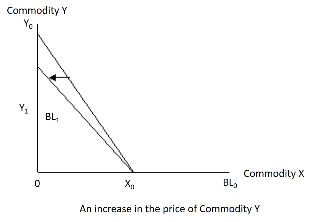
iv) An increase in the price of Commodity Y

 

The budget line rotates inward. The budget line becomes flatter. The opportunity set facing the individual decreases. The individual obtains less Commodity X and Commodity Y.

 

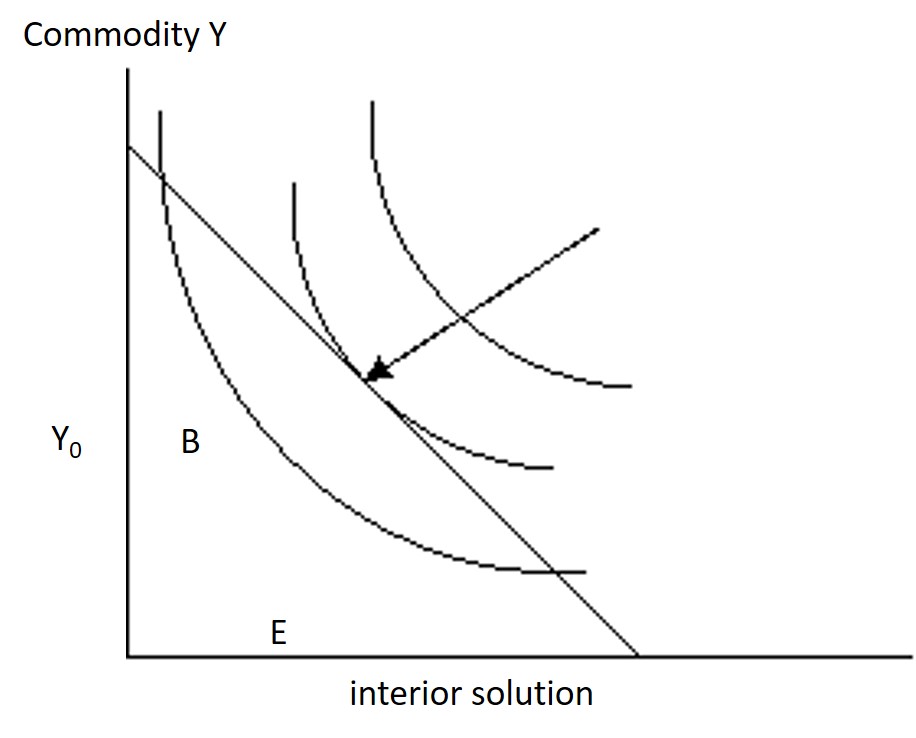
                1) Interior solution

 

An individual maximizes his total utility when the budget line is tangent to the highest indifference curve. An individual will maximize his utility at Point E.

 

At Point E, the slope of the budget line equals to the slope of the indifference curve. That is, Px/Py = MRSxy. At point E, an individual’s consumption decision is at equilibrium.

 

                        For example 1:

Given:

• Px = $8
• Py = $4
• Px/Py =2 (That is, an individual can give up 2 units of Commodity Y for 1 unit of Commodity X.)

 

Suppose:

• At Point B, MRSxy = -4
• That is, at Point B, an individual is willing to give up 4 units of Commodity Y for 1 unit of Commodity X.
• As a maximizer, the individual is willing to buy more Commodity X since the maximum amount he is willing to give up is greater than the market rate of exchange.
• Then, the individual moves down the budget line towards Point E and reaches a higher indifference curve.

                        For example 2:

Given:

• Px = $8
• Py = $4
• Px/Py =2

Suppose:

• At Point C, MRSxy = -1
• That is, at Point C, an individual is willing to give up 1 unit of Commodity Y for 1 unit of Commodity X.
• As a maximizer, the individual is willing to buy less Commodity X since the maximum amount he is willing to give up is less than the market rate of exchange.
• The individual instead will sell 1 unit of Commodity X to get 2 units of Commodity Y.
• Then, the individual moves up the budget line towards Point E and reaches a higher indifference curve.

 

The equilibrium position is called interior solution.

 

Px/Py = MRSxy is a necessary condition for utility maximization but not a sufficient condition for utility maximization.

 

A sufficient condition for utility maximization is that the indifference curve must be convex to the origin.