III.   Use Value, exchange value and the concept of consumer’s surplus

 

A. The concept of exchange value

 

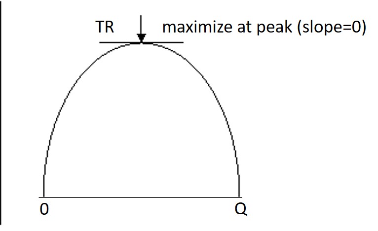
1) What is total exchange value (TEV)?

 

TEV is the total actual amount of other commodities (represented by dollars) that an individual gives up for obtaining certain amount of a commodity.

 

It is the total revenue (TR) received by the producers, so TEV = TR. It is also the total expenditure spent by the consumers

 

2) What is average exchange value or exchange value (AEV)?

 

AEV is represented by total exchange value divided by its quantity demanded. That is .

 

It is the average revenue (AR) received by the producers, so AEV = AR.

 

 

3) What is marginal exchange value (MEV)?

 

MEV is the actual amount of other commodities (represented by dollars) that an individual gives up for obtaining an extra unit of a commodity.

 

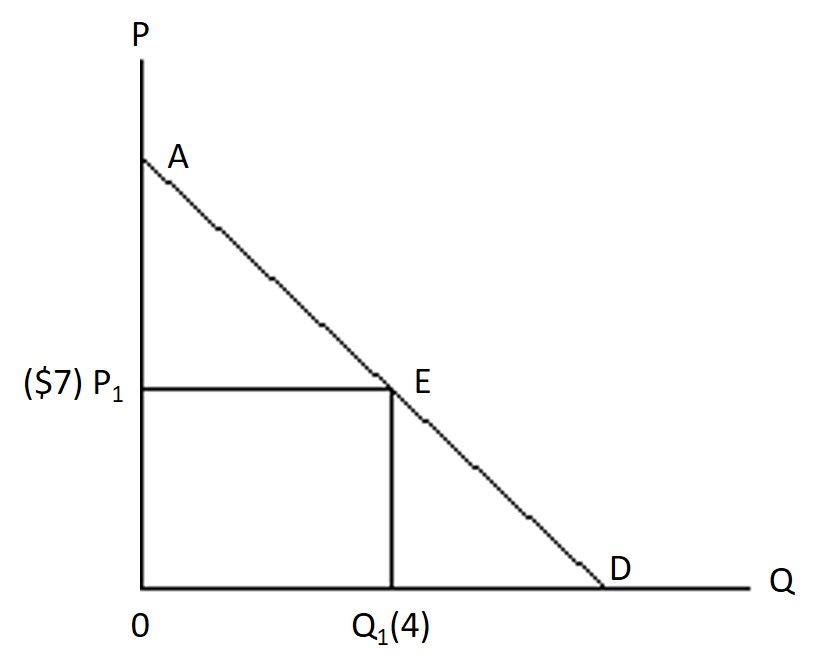
4) Graphical illustration of the concept of exchange value

 

Q	P ($)	AEV($) = P	TEV($) = Q x P	MEV($)
0	0	0	0	-
1	10	10	10	10
2	9	9	18	8
3	8	8	24	6
4	7	7	28	4
5	6	6	30	2

TEV = area OP1EQ1      = OP1×OQ1     = $7 ×4     = $28

 

B. The concept of use value

 

1)          What is total use value (TUV)?

 

TUV is the maximum amount of other commodities (represented by dollars) that an individual is willing to give up for obtaining certain amount of a commodity.

 

TUV = MUV₁ + MUV₂ + MUV₃ + …MUV_n The TUV of 5 units = $10 + $9 + $8 + $7 + $6 = $40. Also, TUV = area OAE Q₁.

 

TUV is increasing when MUV is positive

 

Q	TUV($)	MUV($)	AUV($) = TUV/Q
0	0	-	0
1	10	10	10
2	19	9	9.5
3	27	8	9
4	34	7	8.5
5	40	6	8

 

                

 

2) What is average use value (AUV)?

 

AUV is represented by total use value divided by its quantity demanded. That is .

 

3) What is marginal use value (MUV)?

 

MUV is the maximum amount of other commodities (represented by dollars) that an individual is willing to give up for obtaining an extra unit of a commodity.

 

 

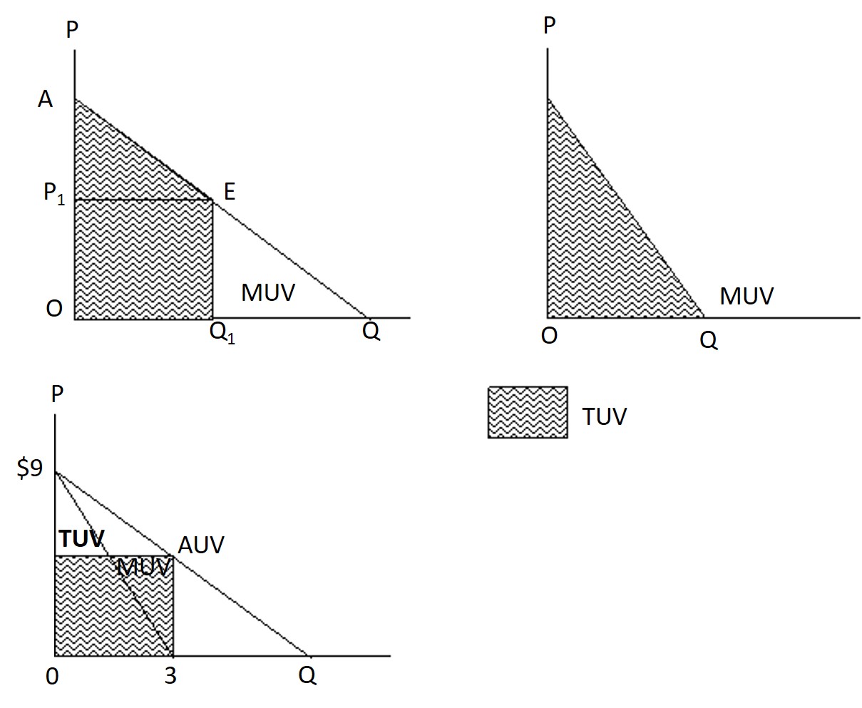
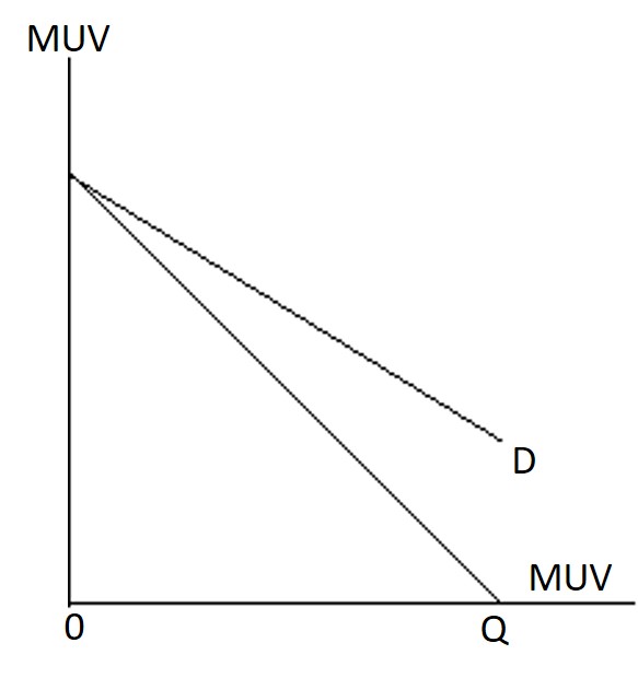
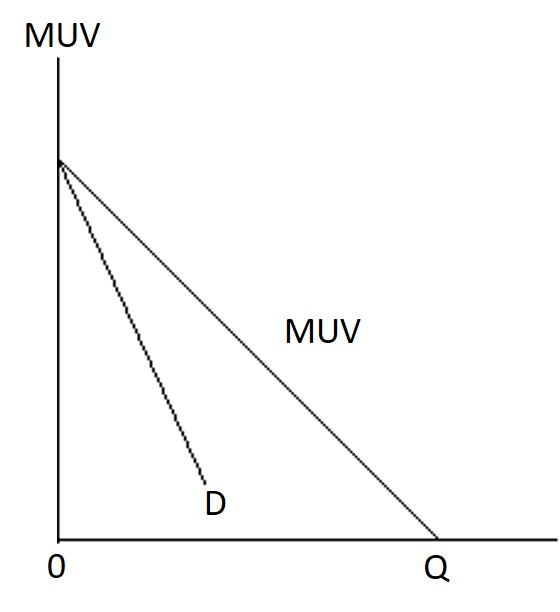
a)     Why MUV curve always lies below AUV curve?

 

        Since                                                

                        

Then

AUV＞OP₁

And

MUV=OP₁

                                Therefore

AUV＞MUV

 

b) What is the law of diminishing marginal use value?

 

The law of diminishing marginal use value states that the maximum amount an individual is willing to pay for a commodity diminishes as more and more of it is obtained. That is why an MUV curve is downward sloping.

 

                        c) What is the assumption of diminishing marginal use value?

 

It is assumed that when an individual has more of a commodity, the TUV of the commodity will be larger but its MUV becomes smaller.

 

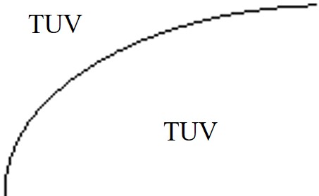
2.6   TUV Curve

• It has a positive diminishing slope (TUV curve’s slope=△TUV/△Q = MUV), reflecting the assumption of diminishing marginal use value

2.7   AUV Curve

• It sloping downward

        2.8   MUV Curve

• It has a negative downward sloping slope
• The Area under MUV curve is TUV
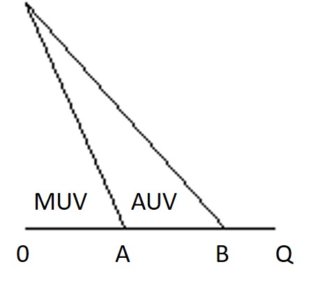
• If AUV curve is a straight line, the MUV curve bisects the horizontal intercept of the AUV curve

 

AUV, MUV                  If AUV is a straight                  line then 0A = AB

3      Concept of Consumer’s Surplus

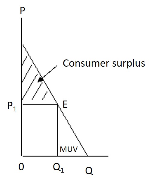
3.1   Consumer’s Surplus

• It is the different between its TUV and TEV
• TUV = consumer’s surplus + TEV
• It is the net gain from exchange (trade)
• Consumers will buy when there is consumer’s surplus
• It is used to derive testable implications to explain different pricing arrangement in the real world
• Many real world pricing arrangements are attempted by sellers to extract consumer surplus

3.2  To find consumer surplus from MUV curve

 

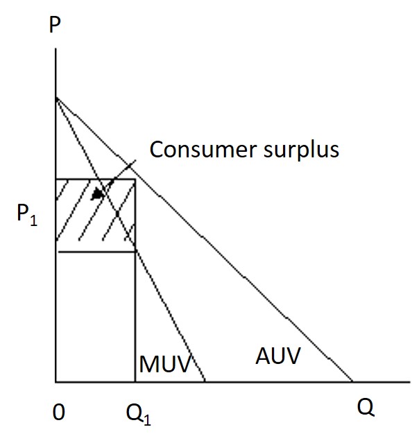
        3.3  To find consumer surplus from AUV curve

 

            

 

4 Basic Assumption in Marginal Use Value Approach

4.1  Each individual desires many commodities and has many objectives

• An individual chooses more than one economic good
• Since the range of economic goods is immense, economic concepts and analysis can be widely applied

4.2  Some commodities are scarce

• Each individual has to choose owing to scarcity

4.3All commodities are marginally substitutable

4.4The assumption of diminishing marginal use value

 

5        Consumer Equilibrium: Using Marginal Use Value Approach

5.1   Consumer Equilibrium Condition

• Gains from exchange arise when the actual amount he pays for the purchase of commodities and services is smaller than the maximum amount he is willing to pay for

 

Q	P	MUV	TUV	TEV	GAIN (TUV – TEV)	NET GAIN (MUV – P) (MUV = P)
1	7	10	10	7	3	3
2	7	9	19	14	5	2
3	7	8	27	21	6	1
4	7	7	34	28	6	0
5	7	6	40	35	5	-1
6	7	5	45	42	3	-2

 

 

• If MUV>P₁, there are potential gains (TUV – TEV) not yet captured. An individual will continue buying the commodity
• If MUV< P₁, there are potential gains not yet captured, There will be net gain (MUV – P) if an individual cuts down his consumption
• To maximize, an individual will consume up to where his MUV = P and net gain = 0

5.2 Equi-marginal Principle

(1) Maximize gain from one source

• To maximize gain, the individual finds the highest or largest value of his total gains
• A firm maximize by finding the highest value on the total revenue curve.
• That is the peak of a bell-shape total revenue curve
• A firm maximize at where the MR=0 or at where the slope of the TR=0

 

(2) Maximize gain from more than one source: equi-marginal principle

• An individual maximize if the marginal gains from all sources of gains are equalized.
• That is MR₁ = MR₂ = MR₃ = ……. MR_n
• Example:
• Suppose teachers in 3 subjects announce that they will hold examinations the day after tomorrow. You figure that the total amount of time you can devote to the study of these three examinations is 10 hours. For each of the examination the relationship between the number of hours you can spend studying and the grade you think you will get is shown below.
• If you want to maximize the sum of your scores in the three examinations, how many hours should you devote to each examination?.

 

Number of hours spent studying	Economics Grade	Marginal Grade per hour	English Grade	Marginal Grade per hour	Chinese Grade	Marginal Grade per hour
0	55	-	50	-	55	-
1	65		60		70
2	75		69		80
3	80		74		85
4	83		79		89
5	85		83		93
6	87		85		95
7	88		86		96
8	89		87		96
9	89		88		96
10	89		89		96

 

• In order to maximize your score in your examinations, you should spend 3 hours on studying Economics; 4 hours on studying English and 3 hours study Chinese.
• The scores gained with the last hour spent on all three subjects are the same and equal to 5 scores.

 

6 Demand and MUV

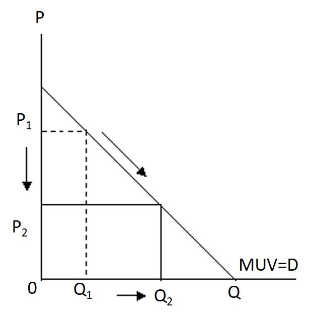
6.1  MUV curve = Demand curve

• The law of diminishing marginal use value states that MUV decreases as more of the same commodity are obtained
• An individual will buy until MUV = P, and MUV is assumed to be decreasing, quantity demanded for a commodity will then increase when the price is lower.
• The above condition is in fact the law of demand.
• Therefore, the law of demand and the law of diminishing marginal use value are identical concepts.
• That is, a MUV curve can be regarded as a demand curve
• The MUV curve is the demand curve as it tells how many units an individual consumes given any level of market prices because:

(1)    Every point on the demand curve represents an equilibrium position since at any given price, an individual will maximize when he consumes up to the point where his MUV = P

(2)    The quantity demanded for a commodity at every price is the result of the maximizing decision of the consumer

6.2   Problem with using a MUV curve as a demand curve

• MUV curve does not consider the effects of a price change on real purchasing power of an individual
• MUV curve only shows the pure substitution effect of a price change. The income effect is ignored
• MUV curve is called real income constant demand curve/income-compensated demand curve.
• The demand curve we learnt before is called money income constant demand curve which contains both income and substitution effect

(1)   If Good X is a normal good, money income constant demand curve will lie to the right of MUV curve

 

                               

(2)   If Good X is an inferior good, money income constant demand curve will lie to the right of MUV curve

 

 

• MUV curve is the demand curve, when income effect is zero because:

(1)    Economists find out that income effect is really insignificant and can be ignored

       (2)    We assume income effect is zero

• The demand curve derived from the indifference curve analysis is a money income constant demand

6.3   Testable implication of demand

• If the cost of raising children increases, the average number of child birth per woman decreases (law of demand)
• The cost of raising children increases because:

(1)   women’s education level increase, i.e. women’s real income has increased

(2)   women’s employment opportunity increase

(3)   costs of employing domestic helper increased

(4)   costs of child caring increased

(5)   costs of educating child increased

• As the price of raising child increases, its MUV increases which means its TUV decreases. That is the quantity demanded decreases.

 

7      Paradox of Value

• Paradox
• Adam Smith finds that it is strange that water has a higher TUV than diamonds but it has a lower TEV than diamonds
• Explanation
• Price or TUV depends on MUV rather than TUV.
• MUV depends on supply.
• Although water has a higher TUV as it is essential to life, its price or TEV is lower since its supply is larger than diamond
• Similarly, diamonds have a lower TUV, its price or TEV is higher since its supply is smaller than water

 

• Error of the paradox
• It is unreasonable to say that water has a higher TUV than diamonds since TUV is something subjective, it is people’ s willingness. The paradox only state rather than derived from the concept of value.
• TEV of water is smaller than diamond can never be verified since they are measured in different unit of measurement

8      All-Or-Nothing Demand Curve

8.1   All-Or-Nothing Basis

• Either an individual buys at the offered quantity and price, or they buy nothing at all

8.2   All-Or-Nothing Pricing Arrangement

 

Q	MUV	TUV	AUV	P	TEV	NET GAIN
1	18	18	18	18	18	0
2	16	34	17	16	32	2
3	14	48	16	14	42	6
4	12	60	15	12	48	12
5	10	70	14	10	50	20
6	8	78	13	8	48	30
7	6	84